New paper – Arctic heat flow

It may be a while since the end of the Arctic Ocean 2016 expedition, but we have just published some new work resulting from the sediment coring efforts in the Journal of Geodynamics. The results from the AO16 expedition were also combined with some newly processed measurements from the earlier 2014 cruise, SWERUS-C3.

While the nice-looking version of the manuscript is behind a paywall, you can find the
pre-print version –> Shephard_etal_2018_Arctic_heat_flow_JGeod,
or email me [g.e.shephard@geo.uio.no] if you would like a copy.

The Earth is cooling. It is losing heat that is/was formed by the radioactive decay of isotopes, as well as from the heat that was formed during planetary accretion. Heat flow thus underpins all aspects of Earth’s evolution and processes including mantle convection and plate tectonics. Heat flow measurements are useful in that they provide a snapshot into the thermal state at a given location. Steady state surface heat flow (whether that be from the seafloor or on land) varies around the world, and depends on a number of factors including the tectonic setting. A number of key papers explaining more about Earth’s heat flow, geothermal gradients and thermal conductivity etc are listed at the bottom of this page.

Globally, heat flow measurements are sparse – but this is particularly true of the Arctic Ocean. A global heatflow database can be downloaded to show a collection of heat flow (be warned, last updated in 2011 – so more recent measurements are missing!).

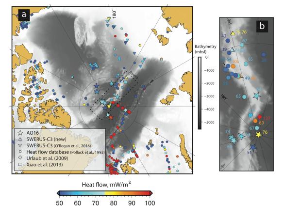
Left: Overview Arctic heat flow measurements. Our new study are the stars and the study of Urlaub et al. (2009) with the high reported values in the diamonds. Right: Zoom into the central Lomonosov Ridge region with reported heat flow values shown.

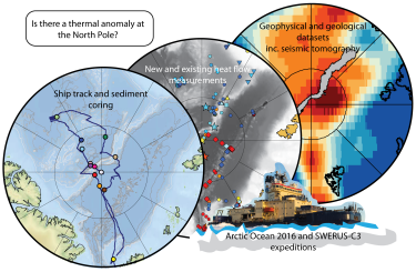
The article presents new heat flow measurements from 15 distinct sites in the Central Arctic Ocean, and compares the results in the context of existing measurements. We have new measurements from the Amerasia Basin (Marvin Spur, Alpha Ridge), the Lomonosov Ridge (crest and foot) and Eurasia Basin (Yermak Plateau and Amundsen Basin). The possibility of a “North Pole thermal anomaly” sounds pretty interesting — we explore surface and deeper mantle evidence, or the lack thereof, for such a feature and its relation to the heat flow measurements.

The results from the three Amundsen Basin sites are pretty interesting in particular because:

• They are the first measurements from that region i.e. “closer” to Greenland where there is the heaviest ice conditions
• They are located on oceanic lithosphere (not on continental rocks, or complicated by later volcanism as with the Amerasia Basin) and thus the heat flow should follow an established relationship according to the age of the lithosphere; heat flow decreases with increasing age of the oceanic seafloor (for 10 Million year old seafloor you can expect 100 mW/m² and for 50 Million year old or more seafloor you can expect half that).
• An earlier study by Urlaub et al. (2009) located further east/north but on roughly the same aged lithosphere found results up to 2 times higher (104-127 mW/m²) than expected from the above relationship – so quite high values indeed.
• However, in contrast, our results (71-95 mW/m²) were broadly in-line with expectations; the greatest deviation was 21 mW/m² higher than expected. At the end of the day they are only three points…a valuable three points, but only three.
• Explaining an apparent spatial variation of heat flow within the Amundsen Basin could come from a variety of sources; seafloor sediments, the structure of the crust, lithosphere and deeper mantle, methodologies, nearby hydrothermal vents, and more, are all things that should be closely considered.
• Two seismic tomography models (method to image the internal structure of the Earth – see my other work here) that were publicly released by other workers show a slow anomaly (typically associated with regions of melt in the mantle, or hot upwellings) located broadly under the North Pole down to around 200 km depth. Albeit located slightly to the east of our sites, this is kind of interesting – does it explain the Urlaub et al. (2009) results at all, or is it related to something else?

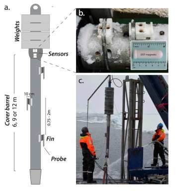
Illustration of the corer setup showing fins with temperature probes and the orientation sensors.

Understanding the thermal and tectonic evolution of the Arctic is still open and what this paper only touches upon can also be used to open up future avenues:

• What is the long-strike crustal variation of the Lomonosov Ridge and how did the Ridge evolve during and since it rifted off the Barents Shelf?
• Is the upper mantle feature identified in seismic tomography ‘real’? What is it – thermal or chemical, or both, in nature?
• What is the role of the ultra-slow spreading along the Gakkel Ridge through time to crustal structure and heat flow?
• A database – oh boy, would an update of Arctic geological and geophysics datasets  in an easy, accessible, updated database be useful. Not a small task though…

Heat flow measurements are a relatively easy and cheap to gather (that is, once you have a vessel and means to send something to the seafloor) and hopefully all future cruises to the Arctic will be able to take such measurements and fill in the gaps, as well as our broader understanding of the geological development of this remote region.

This paper is also special as it is a joint effort of early career researchers who were onboard Oden, and with the guidance of the project supervisors/co-authors at the University of Stockholm, Matt O’Regan and Martin Jakobsson. Thanks again to the Swedish Polar Research Secretariat for the opportunity to go sailing and measuring!

Reference to Article: 
Shephard, G.E., Weirs, S., Bazhenova, E., Perez, L.F. Ramirez, L.M.M., Johansson, C., Jakobsson, M. O’Regan, M., Accepted. A North Pole thermal anomaly? New heat flow measurements from the central Arctic Ocean. Journal of Geodynamics (Arctic Special Issue). https://doi.org/10.1016/j.jog.2018.01.017

References and further reading:

Pollack, H. N., Hurter, S. J., Johnson, J. R., 1993. Heat flow from the Earth’s interior: Analysis of the global data set. Rev. Geophys. 31, 267-280. doi:10.1029/93RG01249

Sclater, J. G., C. Jaupart, and D. Galson, 1980, The heat flow through oceanic and continental crust and the heat loss of the earth, Rev. Geophysics and Space Physics 18, 269–311. doi:10.1029/RG018i001p00269

Stein, C. A., Stein, S., 1992. A model for the global variation in oceanic depth and heat flow with lithospheric age. Nature. 359, 123-129. doi:10.1038/359123a0

Stein, C. A., Stein, S., 1994. Constraints on hydrothermal heat flux through the oceanic lithosphere from global heat flow. J. Geophys. Res.: Solid Earth. 99, 3081-3095. doi:10.1029/93JB02222

Urlaub, M., Schmidt-Aursch, M. C., Jokat, W., Kaul, N., 2009. Gravity crustal models and heat flow measurements for the Eurasia Basin, Arctic Ocean. Mar. Geophys. Res. 30, 277-292. doi:10.1007/s11001-010-9093-x

 Feb 6th 2018, Oslo

New paper – mapping extinct oceans

This week, along with early career colleagues at CEED and at the University of Oxford, we published a paper in the Nature journal: Scientific Reports “On the consistency of seismically imaged lower mantle slabs“. The paper is free for everyone to access, and presents a new and simple method to map out the distribution of features deep in Earth’s interior, namely subducted slabs of ancient oceans.

View of Arctic “slab vote maps” at different depths from our latest study in Scientific Reports. The black and red are the most robust features, the blues less so (grey no slabs).

While this paper might appear as a slight detour from my other Arctic focussed studies, it was partly inspired by work we earlier published about an ancient Arctic ocean that now exists under Greenland. Being a global study, the Arctic can be zoomed into, of course – but keep in mind that the resolution of the data can be a big issue! One of the most exciting aspects of the paper is that there is a companion **WEBSITE** which allows you to recreate the maps and delve into more details. This website will soon be expanded even further to include more options – but watch this space!

Below is a copy of the press release originally posted on the CEED Blog 

 

A novel way of mapping the Earth’s ancient oceans

Deep beneath our feet lies a vast domain that is a record of hundreds of millions of years worth of geological history. A curious image of ancient rock graveyards plunging downwards and hot rising material pushing upwards is not far from the truth. A new study by Shephard et al. published today in Scientific Reports reveals an innovative technique of creating maps that image the interior of the Earth – a ‘colour-by-numbers’ guidebook to ancient oceans that once existed at the surface, if you will.

Earth in motion

The surface of the Earth is in constant motion, with new crust being formed at mid-oceanic ridges, such as the Mid-Atlantic Ridge, and older crust being destroyed at convergent margins, such as around the Pacific “Rim of Fire”. Where oceanic plates plunge into the mantle are termed “subduction zones” (orange lines in the GIF below). Indeed, much of the seafloor that existed when the dinosaurs roamed the Earth has long since been subducted and is now deep in the Earth’s mantle. This constant recycling of oceanic basins means that the Earth’s surface can only tell us so much about the deep geological past – the innards of our planet holds much of this information, and we need to access, visualize, and disseminate it.

Figure/GIF: A plate tectonic reconstruction of the Earth’s oceans from 200 Million Years ago (Ma) to present-day. The grey regions are the continents, the green-blue colours correspond to the age of the oceanic basins (dark is old crust and light is young crust), orange shows the location of subduction zones, the black arrows show the plate velocities and the black lines are the rest of the plate boundaries…. note! non-rainbow colours for the age grids!

Imaging the insides
Using information from earthquake data, seismologists can produce models of the Earth’s interior. Similar to a medical X-ray scan that looks for features within the human body, these “seismic tomography” models image the internal structure of the Earth. However, there are many different types of data that can be used to generate these models, each with varying degrees of resolution and sensitivity to the real Earth structure, and choices in data processing techniques. There are so called P-wave models based on the compressional waves, and S-wave models based on slower shear waves. This variability has led to dozens of tomographic models that are now available in the scientific arena, which all have slightly different snapshots of the Earth. Importantly, the old, cold oceanic plates that have been subducted mean that seismic waves pass through them more quickly than the surrounding mantle (in the same way that sound travels faster through solids than air). It follows that these subducted plates (slabs) can be “imaged” seismically (usually these slab regions are coloured blue in seismic tomography model – see video by co-author Kasra Hosseini).

Which tomography model(s) should be used?
Are models based on P- or S-waves more likely to pick up a feature?
How many models are sufficient to say that a deep slab can be imaged robustly?

Voting maps
To facilitate solutions to these questions, a novel yet simple approach was undertaken. Different tomography models were combined to generate counts, or “votes,” of the agreement between models – a sort of navigational guidebook to the Earth’s interior. A high vote count means that an increased number of tomography models agree that there could be a slab at that location. For the study in Scientific Reports the focus was on slabs in the lower mantle (700-2850 km depth) but the process can be undertaken for shallower depths, and for other features such as mantle plumes. The maps show the distribution of the most robust slabs at different depths – the challenge is to now try and verify the features and potentially link them to subduction zones at the surface back in time. Many studies have started to undertake a similar exercise on both regional and global scales, but these vote maps can now serve as an easy resource for the community to continue this task.

Secrets in depth

When viewing the vote maps either on a surface map projection or as a vertical slice, many interesting features are displayed. A bit like dessert-time discussions about the best way to cut a cake, so too are the ways of imaging and analyzing the Earth. Do you slice it horizontally and see things that might correspond to the same age all over the globe? Or slice vertically to see a spectrum of ages (depths) at a given location? Or perhaps the 3-D rendering a volumetric body would be most insightful?

Figure: Vote maps loaded into GPlates software showing different imaging options for the region under Southeast Asia.

By comparing the changes in vote counts with depth, some intriguing results were found. An apparent increase in the amount of the slabs was found around 1000-1400 km depth. This could mean that about 130 Million years ago more oceanic basins were lost into the mantle, or perhaps there is a specific region in the mantle that has “blocked” the slabs from sinking deeper for some period of time. This observation and numerous other amazing features revealed by our new maps have already lead to discussions with researchers in plate tectonics, mantle dynamics, and mineral physics.

A resource for the community

Figure: Snapshot of the online “vote map” website where the user can recreate and analyse the vote maps further. https://www.earth.ox.ac.uk/~smachine/cgi/index.php

Having accessed the different tomography models provided by different groups or repositories, this study was facilitated using open-source software (Generic Mapping Toolsand GPlates). An important component of reproducible science and advancing our understanding of Earth is to make datasets and workflows publically available for further investigations. An online toolkit to visualize seismic tomography data is being developed by the co-authors and a preliminary vote maps page is already online. Here, vote maps for a sub-selection of tomography models can be generated, including with a choice in colour scales and with overlays of plate reconstruction models. More functionality will soon be available – so watch this space!

Shephard, G.E.(1), K.J. Matthews(2), K. Hosseini(2), M. Domeier(1). 2017. On the consistency of seismically imaged lower mantle slabs. Scientific Reports, v.7. doi:10.1038/s41598-017-11039-w
1. Centre for Earth Evolution and Dynamics (CEED), University of Oslo.
2. University of Oxford.

Post AO16 – reflections and next steps

After a hiatus from posting to this blog – I thought to post a summary of what we achieved during Arctic Ocean 2016 in the sediment coring team, and what the next plans for the many meters of mud are. So, 47 days at sea on an icebreaker… what did we achieve? A muddy well lot.

Photo: Looking back towards the Canadian icebreaker, Louis S. St-Laurent, trailing in the path cut by Oden. You can see the yellow “A-frame” on the aft deck which was used in the coring procedure.

I was part of the sediment coring team which included the onboard work package leader Carina Johansson and coring technicians Markus Karasti and Draupnir Einarsson, all based out of the University of Stockholm. The project was overseen by Martin Jakobssen (Uni. Stockholm) who was shorebased for the expedition. My fellow early career researchers were PhD student Steffen Wiers (Uppsala University), who works with palaeomagnetics, and Luz María Mejía Ramírez (Universidad de Oviedo), who works with microfossils and is now based the ETH in Zurich. A truly awesome team – and I might add, reigning icebreaker “Dance Off” champions.

Photo: Coring team at the North Pole (L-R; Wiers, Shephard, Einarsson, Johansson, Mejía Ramírez and Karasti)

A total of 13 sites were successfully sampled from the Arctic Ocean, each with a relatively unique oceanographic and geologic setting. We ended up going to all of the target areas discussed in the sites of interest blog entry, and more. There were two main types of corers used; a piston corer (up to 9 or 12 m), and a gravity corer (up to 6 m). Unlike the gravity corer, which works largely under its own weight, the piston core, uses yep, a piston. This makes it more ideal for capturing longer sections, especially in softer sediments, and not disturbing the contents as much. It also requires the use of a trigger weight, to which short corer (itself a gravity corer, up to 3 m) can be attached leading to a sort of “core one, get-one-free” kind of deal with a piston core.  At the 13 sites (a 14th site was unsuccessful) we recovered 21 successful cores (piston, gravity, and/or trigger), which translated to 111 m of sediment.

The sediment coring onboard process can be largely divided into main steps; preparation, coring, logging, splitting and describing, sampling, and packing. A lot of work had gone into setting up the equipment and workflow before we set sail, as well as transport and storage of the sediments after the cruise (not to mention the impending science to be done!). We did not have shift work per se, but some days we were coring at 3 am and sometimes working 12+ hours, but that is the nature of such an expedition and the samples were not going to collect themselves!

Figure: Locations of the 13 successful coring sites (site #14 was unsuccessful).

1. Preparation: Firstly, the actual coring site needs to be decided upon, and this relies on coordination with the bathymetry and geophysical imaging mapping team who have real-time images of the seafloor. Some of the deciding factors as to where and when we core include sediment thickness, any nearby seafloor structures like rocks or slopes, the weather and ice conditions and of course the science questions you hope to answer. Additionally the core-type (piston or gravity) needs to be selected and rigged up. There are lead weights placed on the top of the cores, and for the piston core it weighs typically 1400 kg, and 800 kg for the gravity core. Furthermore, each of the corers has a PVC liner which needs to be marked in advance so that when it is full of sediments and cut into sections we can find out the order of the sections, and what is up and what is down (retaining the orientation is very important!). Probes can also be attached to the outside of the corer to measure the temperature of the water and the sediments during the trip and will provide valuable “heat flow” data.

Figure: Image of the sediments from the “sub-bottom profiler” at Site 6 (red rectangle) – the North Pole. The light and dark lines indicate relatively undisturbed, flat sediments. (Image: L. Perez GEUS)

2. Coring: The corers are attached to high strength wires located on the aft deck (back of the ship) and descend to the seafloor at a rate of about 1.5 metres per second. When working in 800 m water depth this translates to about 20 minutes up/down time, but in 4000 m the waiting time on deck is around 1.5 hours. Once the sediments are captured in the corer, it is brought back up to the aft deck and the liners are pulled out from the corers. The initial pull-out force required to start the ascent with the corers full of sediment can be in excess of 6000 kg(f).  Once on deck they are cut into manageable 1.5 m sections (water logged sediments can be quite heavy) and carried up to the lab deck at the other end of the boat.

Photo: Left, looking down on to the aft deck during piston core retrieval and right the all important winch to which the core is attached.

3. Logging: The cores (now I refer to the white liners with sediments) are stored vertically and left to rise to room temperature for about 24 hours. The segments are then logged for geophysical properties i.e. non-invasive techniques, using the MSCL or “Multi-Sensor Core Logger”. This gives a first exciting glimpse into what might be inside. These properties include P-wave velocity, gamma (bulk) density (which used a radioactive 137Cs source, no touchy), magnetic susceptibility and colour line-scan imaging. In the Arctic Ocean these measurements can often be compared across vast distances to other cores from other expeditions and give a basis for “correlation” which is relevant for assigning times and palaeo-settings. Sometimes pore water was sampled at this stage by sticking syringes with porous membranes into the liners.

4. Splitting and describing: After the logging is completed the core sections are then taken to the splitting tent where the liners are split lengthways and opened, revealing the muddy treasure. They are then returned to the main lab where they are carefully scraped to reveal the layers and then described by hand/eye on a cm-by-cm scale. The descriptions include details such as structure, grain size, deformation and colour. Sadly the classic “baby poo brown” is not a valid descriptor, and RGB-based colour charts are used to help with the subjectivity of that task. If a stone or shell was found this was also noted. To be fair, not all the sediments were shades of brown/grey/black as we did find some spectacular goldish yellow, greenish, pink and even blue muds. Finding a variant of this coloured mud was a particularly good day (a month+ has passed since my last mud sample, so I can enthusiastically reminisce about it). Additional physical properties can also be measured at this point including thermal conductivity, shear strength and pH.

Photo: Left to right: sections from one core all lined up; plastic cubes used for palaeomagnetic sampling; and thermal conductivity measurements.

5. Sampling: Because the core has been split length-ways there are two nearly identical halves. One becomes the “working half” which sees all of the sampling action, and the other the “archive half” which serves as a half to which we can return to in the future. On this cruise we were sampling for a few things including a proxy for sea-ice and palaeomagnetics. We were also on the hunt for microfossils including diatoms and foraminfers, but these are a little harder to spot. Samples were taken every 2-4 cm along the entire length of the core, and were bagged and tagged, and some were then frozen. The sampling process for each core took around 1-2 days.

6. Storage and next steps: Once we were finished with the cores, they were tightly wrapped in plastic (exposure is not ideal for preservation) and placed in large plastic tubes for storage. Since the end of the cruise, the cores and samples have made their way back to Stockholm where they await further analysis. One of the great things about sediment cores is that they contain a lot of information and will potentially lead to a lot of great science.

You can watch a summary video of the coring experience below (in English)

So what are the results from the AO16 sediments? It is a bit early days to tell as they will be undergoing further analysis with extra instruments now that they are back on land. But we saw very clear periods of glacial (lots of ice) and inter-glacial (not so much ice) times, which was most easily identified by a change in colour. We saw periods where the sediments were a lot coarser and sandier e.g. “sandy silt”, which means that it was more of a coastal environment, and other periods with very fine e.g. “mud” or “silty mud” which indicate a calmer, low energy environment. Sometimes the sections were very long and homogenous whereas other times they had high-frequency and thin banding. The boundaries between sediment layers were sometimes very blurred and difficult to identify, perhaps indicating a gradual change in environment, whereas other times they were very sharp, pointing to a faster change or rapid event. We might have recovered sediments back to “Marine Isotope Stage 6” which started around 200,000 years ago – but time will tell 🙂

During the cruise I was able to post to my twitter account based on the onboard email setup (check out the “recipes” at IFTTT if you find yourself without the interwebs), so you are able to check out some more of the photos. You can also read Carina’s nice blog with many photos which she posted to from Oden, in Swedish here.

My eternal gratitude and appreciation goes to the whole crew of Oden, the Swedish Polar Research Secretariat and their Early Career program, Carina and the sediment coring team, and all of the science party onboard Oden and the Louis. 

01 November 2016, Oslo

Day 1 – Longyearbyen

Hi all, a quick update on Arctic Ocean 2016 activities having now left solid ground. The large international scientific contingent landed this afternoon at around 15h on a flight from Oslo-Tromsø-Longyearbyen.

Day 1 (2100h)
Location: 78° 14.20’N and 015° 39.13’E
Speed: 0.0 kts
Air Temp: 5°C
Water: 6.5 °C
Choccie stash levels: 99.5%

Photo: View from the deck of Oden back towards Longyearbyen

The icebreaker is currently anchored a few hundred meters out from the docks which provides nice views back to the town. This also means I can tap into the last of the norwegian 4G network before anchors-up at 0800h tomorrow. Apparently it will take about 24 hours to reach the ice edge (aka the realm of the polar bears). This will be the toughest bit in terms of waves and potential sea-sickness as it is open water, but once we are in the ice it is mostly vibrations and a minor bit of rolling that can be expected. Between information meetings and another fire safety drill we also had a flying visit from the Sysellmannen (Governor) of Longyearbyen in a helicopter  and we will rendezvous with les canadiens over the next 24-48 hours too. We have been issued with personal “COBS” phones to which we can call anyone on the ship (or everyone if we press the wrong button). There is also an internal Wifi system and a server to which we can share files with others onboard and see key ship stats. Apparently there is a microwave datalink that will be set up between the two ships as well. At midnight (still the midnight sun this far north!) tomorrow we will also switch timezones to UTC for the remainder of the trip. Excellent food so far, and I have not frequented the onboard gym or two saunas as yet.

Photo: View from the bow looking up to the bridge. Blue containers are where we will be cutting and sampling the core.

We also have rather comfortable living quarters with 4 person shared bunk-style rooms. I am located in a room portside towards the bow of the ship. Work hours, for those not on shift work, will probably revolve around meal times which are strictly set and include three square meals and two “Fika” or coffee breaks. Not one to differ from their Norwegian neighbours, the Swedes also prefer a rather early, ahem 1730h, dinner time.

That is all for now – my Twitter @ShepGracie might have more activity now that I see how the email is set up. Goodbye internet and hello Arctic Ocean.

Photo: From within the engine room. Can’t imagine how loud it will be when we are out in the ice!

08 August 2016, Longyearbyen

Arctic Ocean 2016 Sites of interest

This is the second Arctic Ocean blog (following the Overview post) and explains a little more about where we are heading and the type of features we are targeting. 

The seafloor, with its underlying sediments and rocks, is not as boring as it may seem. The Arctic Ocean may be the world’s smallest ocean but by no means does that translate to a simple evolutionary history – it is commonly said that we understand more about the surface of Mars than we do about our ocean floors. The Arctic Ocean is surrounded by shallow and largely flat continental shelves, and has a deep and undulating interior. It is in this central area where many aspects of geology and oceanography become particularly exciting, and where we are heading on Oden.

Figure: Overview of the Arctic Ocean topography and bathymetry (IBCAO) with major features labelled: AB Amundsen Basin, CP Chukchi Plateau, MJ Morris Jesup Rise, MS Marvin Spur, NB Nansen Basin, YP Yermak Plateau. The Lomonosov Ridge separates the two major basins of different ages and red box shows the general area of the cruise sampling sites.

The Arctic Ocean today is the culmination of a long history of horizontal and vertical plate motions; there have been plate collisions leading to mountain building events and/or subduction events where some rocks are pushed deep into the mantle, rifting between plates and the opening of new ocean basins, changes in sea-level, periods of glacial or greenhouse conditions as well as volcanism on massive and localized scales. The dynamic and intrinsic interplay between the geosphere, biosphere, atmosphere and hydrosphere is particularly pertinent in understanding the evolution of the Arctic. The sedimentary record (or “stratigraphic record”) can tell us a lot about the many geologic and oceanographic processes that have occurred within the Arctic – at least as far back in time as we can retrieve from the samples.

Figure: International chronostratigraphic chart (time, basically) which shows the names of the time periods we refer to, as well as their absolute ages – geoscientists often switch between names and numerical ages. On this cruise we will be looking at sediments from the first column, especially the last Quaternary period and hopefully the Cretaceous. Figure from the ICS webpage.

The Arctic Ocean consists of two major ocean basins; the Eurasia Basin in the eastern domain and the Amerasia Basin in the western domain. The long, thin Lomonosov Ridge separates the two basins which are of significantly different age. The opening of the long, linear Eurasia Basin is relatively well understood – spreading occurred around 55 million years ago (‘Ma’ or ‘Myrs ago’) along the Gakkel mid-oceanic ridge and is continuing today at a very slow rate of around 1 cm/yr. By contrast, the Amerasia Basin is thought to have opened over 100 million years ago and the style and timing of opening is hotly debated in the geoscience community. Part of this complication is related to several large bathymetric features of uncertain origins – some features are thought to include continental rocks, others oceanic rocks, and others a kind of transitional type or related to massive volcanism. In addition to physical sampling including coring, dredging and heatflow measurements, other methods to investigate the sub-surface structure of the region include gravity and magnetic measurements, as well as seismic waves and acoustic sound data.

GIF below: Simplified plate reconstruction (fixed Eurasia for reference) running from 160 million years ago to present-day showing the rotation and opening of the Amerasia Basin between 160-120 Ma followed by the Eurasia Basin from 55-0 Ma. You can also see some rifting and spreading between Greenland and North America and Greenland and Eurasia. Present-day topography is reconstructed and plate boundaries are in black. Base reconstruction is from Shephard et al. (2013; Earth Sci Reviews) and is visualized in the freely available software GPlates.

Below I summarize a few key structural features from the central Arctic relevant for the cruise. These features have variable rock types and ages as well as different thicknesses and ages of the overlying sediments. Generally speaking, some of the sediments are nice and flat, capturing a near continuous record of time, and are referred to as “conformable.” Other sites may have been disturbed by ice, water currents, have slumped down from a slope or been uplifted and exposed to sub-aerial erosion, and/or have been disturbed by tectonic motions through time.  On the cruise we aim to sample sediments of all ages from within the basin, and I am particularly interested in as old as possible.

Lomonosov Ridge: Slither of continental rock that rifted from the edge of Eurasia (e.g. the Barents Shelf) with the opening of the Eurasia Basin around 55 Myrs ago. There have been a number of expeditions to sample this feature including sedimentary coring samples and the only deep sea-drilling core ACEX. Both Russia and Denmark (Canada is yet to resubmit…) have submitted claims under UNCLOS covering parts of this ridge.

Alpha-Mendeleev Ridge: An extensive feature that broadly stretches from north of the Canadian Arctic Islands to the Russian shelf. Proposed to be part of the High Arctic Large Igneous Province that erupted around 120-90 Myrs ago. Whether the Alpha and/or the Mendeleev Ridge(s) includes, or is underlain by, continental or oceanic rocks is unclear – it is a key feature in understanding the opening of the Amerasia Basin. This is a site where we hope to recover some of the “older” sediments i.e. Cretaceous age ~ older than 66 Myrs. In particular we will re-visit some sites from the 1960-80’s T3 and CESAR expeditions.

Marvin Spur: This looks like a mini-me of the Lomonosov Ridge and might include some undisturbed sediments of Quaternary age. It is likely related to the same rifting event that opened the Eurasia Basin, even though it is located on the Amerasia Basin side of the larger Ridge.

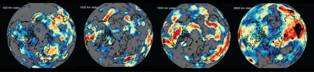
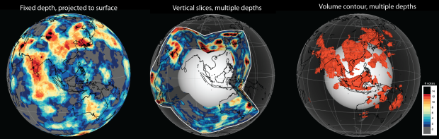
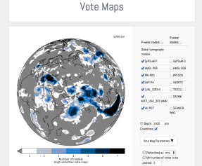
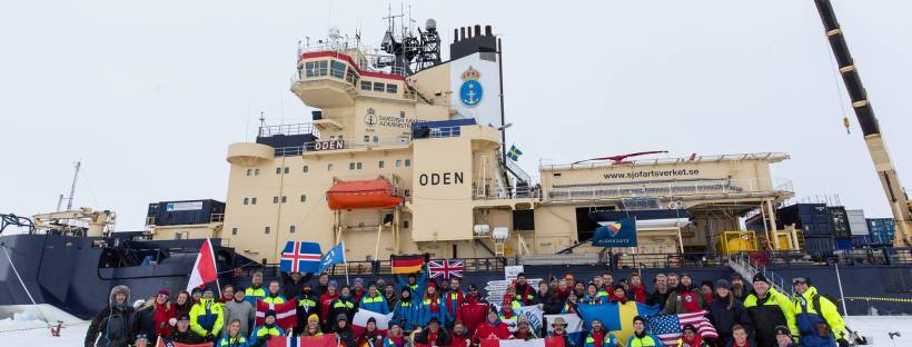
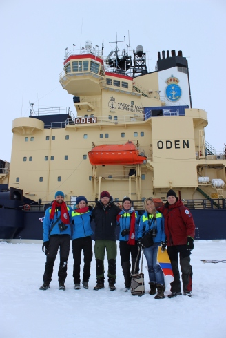
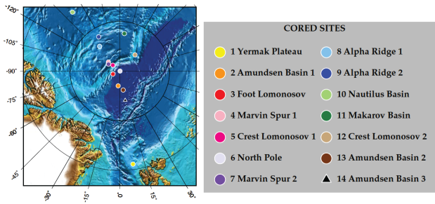
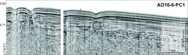
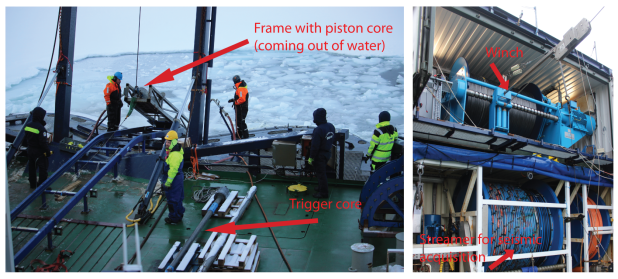
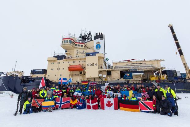
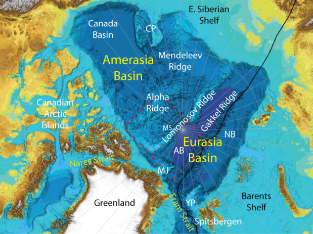
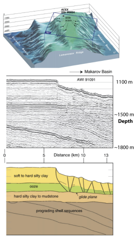
Figure (right): Figures reproduced from Kristoffersen et al. (2007; Marine Geology) showing zoom into Lomonosov Ridge (top), sample of acoustic stratigraphy (middle; from AWI-91091) and interpretation of sediment type (bottom).

Canada Basin: Restricted region of the larger Amerasia Basin. Recent studies suggest that this is the only region of “true” oceanic seafloor. Prevailing models favour a counter-clockwise rotation of Alaska and parts of Russia away from Canada sometime around 140-100 Myrs ago. While we will not be sampling this area, considering the relationship between the Canada Basin and the remainder of the Amerasia Basin (especially the Alpha Ridge and the closest side of the Lomonosov Ridge) is critical for creating holistic regional models.

05 August 2016, Oslo

References:
–Kristoffersen, Y., Coakley, B., Hall, J.K., and Edwards, M. 2007. Mass wasting on the submarine Lomonosov Ridge, central Arctic Ocean. Marine Geology v.243 p.137-142.
–Shephard, G.E., Müller, R.D., Seton, M. 2013 The tectonic evolution of the Arctic since Pangea breakup: Integrating constraints from surface geology and geophysics with mantle structure. Earth-Science Reviews 124, 148-183

What’s in a name – Arctic Koala

While thinking of the blog name ‘Arctic Koala’ I was struck by a nice little bit of coincidence and thought to share it with you.

Arctic: Choice was easy given my current research interests, upcoming expedition destination and general predisposition the exoticness and remoteness of it all. Arctic derives from ἄρκτος or “arktos” meaning “bear” in Greek. Unlike its furry counterparts, this in reference to one or both the constellations that are visible in the Northern Hemisphere; Ursa Major aka the ‘Great Bear,’ or the Ursa Minor aka the ‘Little Bear.’ The reference to bears is thought to come from a mythological story regarding Zeus. In an additional twist, Ursa Minor is Latin for ‘Smaller She-Bear.’ The Little Bear contains Polaris, the North Star (also referred to as the Polar Star), which is close to the north celestial pole. It follows that Antarctic is the “anti” to the Arctic.

Photo: Koala at the Australian Wildlife Park north of Sydney.

Koala: Well, I love koalas, everybody loves koalas. They are one of Australia’s most iconic and seemingly cuddly (and yet have your heard them scream/growl? or seen their claws?) animals and happen to look like mini bears, kinda. While they are not technically bears and are the only extant member of their Family, let’s not let facts in the way of a good symbolic moment. The scientific name for them is Phascolarctos cinereus – and you will notice the “arctos” component, as above, and Phaskolos meaning “pouch.” While we are on the topic of etymology – “Koala” derives from the Indigenous Australian Dharug word gula. 

So indeed there is a little she-bear component in the Arctic….and I think that a Koala, albeit from the southern hemisphere, is as good a representative of a little bear as any. I also found an independent blog post drawing parallels between the koala and the ‘Great’ polar bear (Ursus maritimus) in terms of fur insulation, you can read that one here.

And there you have it, Arktos (Phascol)Arctos!

04 August 2016, Oslo

Arctic Ocean 2016 Objectives

Why am I off to the North Pole, you ask? Isn’t Norway far enough from Australia? This first blog post is a summary of some of the overarching objectives and themes for the expedition.

For the 43 days following this coming Monday, the 8th August, I will be onboard the Swedish Icebreaker Oden – for science! I am part of a ~60-strong team onboard Oden, including scientists and crew. We will be departing and returning to Longyearbyen, which is the main settlement on Svalbard, the largest island in the archipelago of Spitsbergen. Located at 78.2°N, we will indeed already be in the Arctic before we set sail!

Photo: View over Longyearbyen township looking towards the east, during my first visit to Svalbard in August 2015.

We are heading north towards the region of the Amundsen Basin and northern Amerasia Basin in order to target a number of bathymetric features, both by direct and indirect sampling methods. Below is a map of the general region to where we will be travelling. I am one of nine early career scientists invited by the Swedish Polar Research Secretariat, and am working within a sedimentary coring team which will work closely with a geophysical mapping group. This area is one of the most remote regions on the planet and holds many clues as to the geological evolution of the wider Arctic, as well the Arctic Ocean’s place within the global ocean network. There are several other scientific projects running in parallel (its not just rock and mud-loving geologists!) and I will follow up with another post on those soon. You will see that we are working in water depths in excess of 3000 m and in a region with bumpy seafloor terrane, which presents multiple technical challenges. Longyearbyen is located ~1,310 km from the North Pole which is comparable to the distance between Melbourne and Brisbane – probably won’t see any arctic kangaroos on this route though.

Figure (below): General Arctic Ocean 2016 expedition area and
Longyearbyen marked with star (IBCAO grid).

This polar expedition is a collaboration between the Swedish Polar Research Secretariat and the Canadian Government (via the Canadian Hydrographic Service, Natural Resources Canada and the Canadian Coast Guard). The overarching Canadian aim is related to their submission to Commission on the Limits of the Continental Shelf, which is part of the UN Convention on the Law of the Sea (UNCLOS). A submission goes through a lengthy review process, including considerations of neighbouring states’ claims – the conclusion of which may effectively extend a state’s jurisdiction over the continental shelf. The lead scientist (onboard Louis S. St-Laurent) is Mary-Lynn Dickson from Natural Resources Canada and the co-lead Scientist onboard Oden is Katarina Gårdfeldt from Chalmers University of Technology, Sweden. The official cruise blog and “Arctic Portal” along with further info can be found here.

The expedition will involve two icebreakers, Oden and its Canadian counterpart Louis S. St-Laurent, with data acquisition occuring on both of them.

Oden (call sign SMLQ):

•  Built in 1988
• Length of 107.8 m and beam (width) of 31.2 m (more tech specs).
• It can travel at around
  • 16.0 knots max (29.6 km/h; 18.4 mph) in open water
  • 3 knots (5.6 km/h; 3.5 mph) in 1.9 m of ice
• 24 500 horsepower

The Louis S. St-Laurent (call sign CGBN) is slightly older (built in 1966) as well as longer and thinner, at 119.8m by 24.38m (more tech specs). The ships will meet along route somewhere and there will be a helicopter on each ship. Being my first time onboard an icebreaker (excluding the often boozy pre-conference events that share the same name), and my first fieldwork trip in several years, witnessing the various ship operations and real-time data collection will certainly be an eye-opener. I apologize for any technical, or otherwise, inaccuracies in advance. This website has been useful for tracking the realtime locations of the ships but I am unsure how far north it will be able to track given the limited satellite coverage.

What is not shown in the topography and bathymetry map above is the ice coverage – and of course, that is the reason why you need an impressive ice-breaking vessel to travel to the North Pole. One of the reasons this part of the Arctic Ocean is so poorly understood is because it has some of the thickest and most persistent ice coverage, even in the aftermath of summer. Below is a map from this website which shows some the latest sea ice thickness and coverage as of the 2nd August 2016. You will see that there are regions of ice >4 m in thickness – this will be a factor determining the eventual ship track and sampling locations.

Figure: The large map shows the sea ice thickness in the Northern Hemisphere. Inset shows the yearly variation of the sea ice volume in the Northern Hemisphere. Updated daily and used from http://polarportal.dk/en/havisen-i-arktis/nbsp/sea-ice-extent/#tabs-1

Undertaking fieldwork is usually very expensive, let alone conducting it from within the central Arctic Ocean, and therefore being able to participate in such an exciting research expedition is wholly dependent on securing funding and/or scholarships. I would like to end this post by thanking the Swedish Polar Research Secretariat for the opportunity and the initiative shown towards early career scientists.

03 August 2016, Oslo

Test blog

This is a test

123